2015-April-15 Lab 14: Impulse-Momentum Activity

PURPOSE:  To verify that the impulse-momentum theorem holds true during three different collisions.

MATERIALS: 

• Cart with a spring plunger contraption (plastic spring bit can be pushed in and springs out)
• Second cart that moves on a track

PROCEDURE:

Experiment 1:

• Set up track with a moving cart on one end, with force sensor placed on top
• Replace the hook of the force sensor with a rubber stopper 
• Clamp stationary cart (with spring plunger attached) to a rod clamped to the table on the other end of the track (see below)
• Set up so that spring plunger and rubber stopper hit one another during a collision
• The motion sensor should be placed on the end of the track opposite the stationary cart

• To begin the experiment, we opened a pre-setup LoggerPro file called Impulse and Momentum, and made sure to calibrate and zero the force sensor
• To run the experiment, we simply pushed the cart towards the spring plunger and let it bounce back
• The data we got from this experiment was graphed on two graphs:
• Velocity (m/s) vs. Time (s)
• Force (N) vs. Time (s)

The first graph from above shows velocity of the cart before it hits the spring plunger, while it is hitting, and after it bounces back.  Using this data, we can find the change in momentum of the cart.  Before the experiment, we measured the mass of our cart to be 0.640 kg.  We used the examine tool to find the velocity of the cart before collision and after collision and plugged it into an equation for change in momentum:

The amount of momentum change resulted in 0.585 N s.  According to the impulse-momentum theorem, the change in momentum for the moving cart is equal to the total impulse acting on the cart.  The total impulse can be found by taking the area under the force and time graph during the collision.  In our situation we used the integration tool to integrate Force x time during the collision, and found the area to be 0.5442 N s.  These results show that our change in momentum and net impulse are within 7% of each other.  

Part of why this is off could be because the before and after velocities of the cart varied.  This could be due to an imperfect spring bumper that causes an elastic collision that is not perfect.  It could also be due to variations in the track.

Experiment 2:

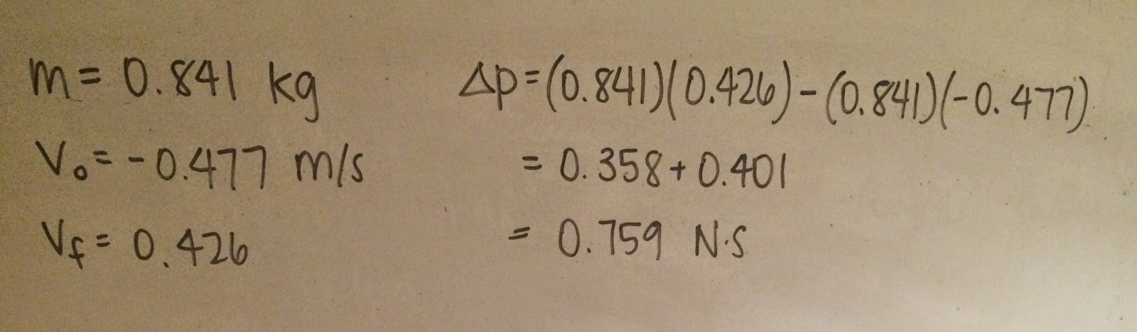
For the next part we added 200 grams to the cart and then ran the same experiment to collect the following data:

Again, we found the total impulse by integrating the force x time graph during the collision.  This value was 0.6998 N s.  We also calculated the change in momentum using initial velocity, final velocity, and mass:

Change in momentum resulted in 0.759 N s.  Impulse and change in momentum were within 8% of one another.  Using a more massive cart made impulse and change in momentum less equal to each other by a small amount.  However, this should not have been the case.  They should have been consistently equal to each other in both experiments because the mass of the cart stays the same during the collision.  The results may have been off again in this experiment due to the same factors that were caused in the previous.

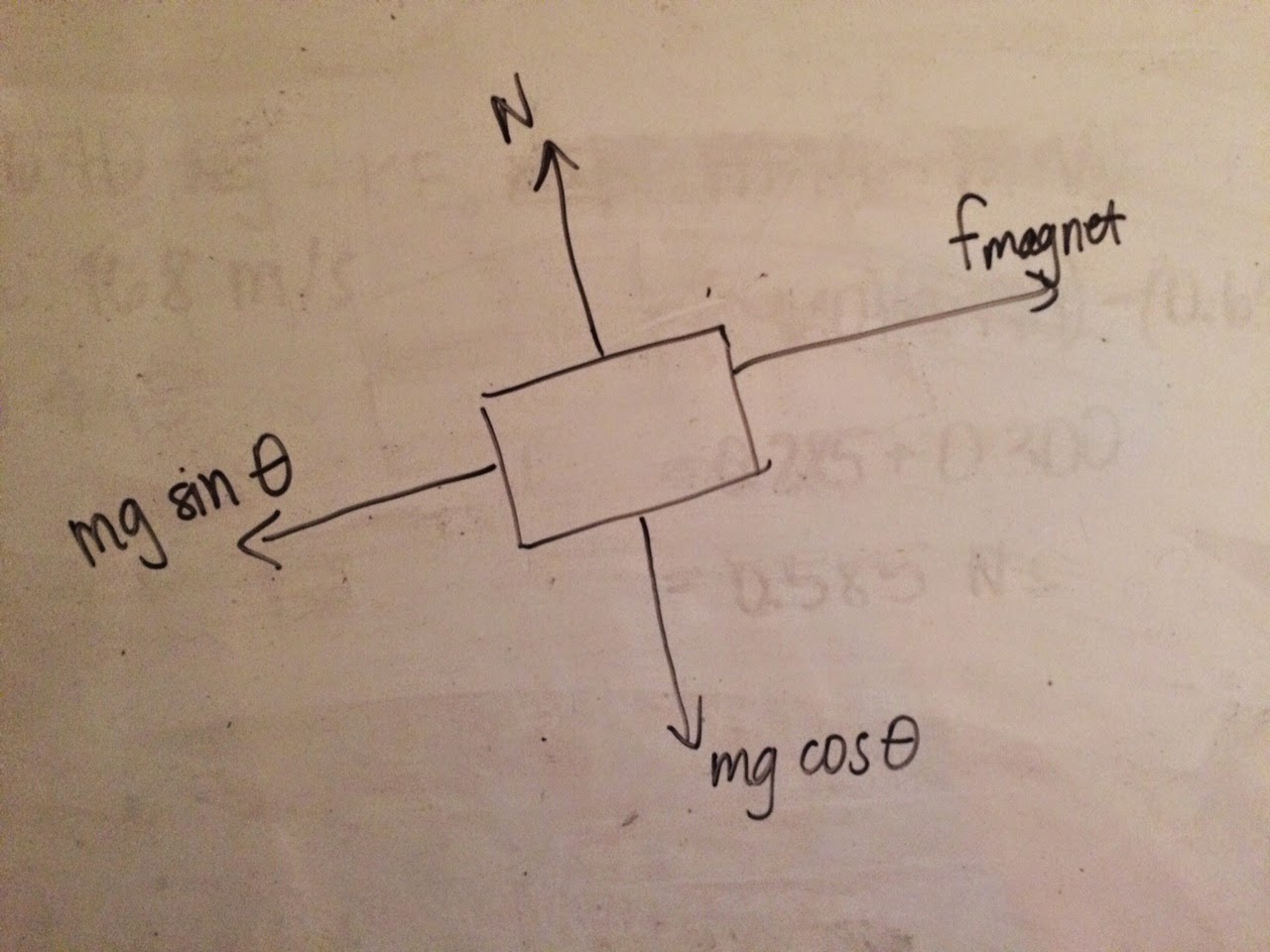
Experiment 3:

For the last trial, we replaced the stationary cart with a block of wood that had clay attached to it, and replaced the rubber stopper with a nail.  This causes an inelastic collision on impact.

We ran the experiment, and the cart comes to rest after the collision.  We obtained the following data:

Again, we found the integral for the period of collision, which was 0.3869 N s.  Calculating change in momentum, we have: 

Change in momentum, with final velocity as 0.

In this situation, the results again are within 7% of each other.  We predicted that even in the inelastic collision, impulse and change in momentum would equal each other.

We can also notice that impulse in this inelastic collision is about half the impulse of the elastic collision with the same mass.  We had predicted that the impulse would be less for the inelastic collision because it is over a shorter period of time.  

CONCLUSION:

In all three experiments (1) elastic collision with some mass, (2) elastic collision with greater mass, and (3) inelastic collision with greater mass, the impulse and change in momentum were nearly equal to each other.  Impulse and change in momentum are greater when using a larger mass.  Both are also about half the value during an inelastic collision, because the time span for an inelastic collision is smaller.

Our results were about 7-8% in error, which could have been caused by nicks or uneven parts of the track, altering the initial and final velocities.  The spring that we used may not have been of the highest quality.  

2015-April-13 Lab 13: Magnetic Potential Energy

Magnetic Conservation of Energy

Jenna Tanimoto

Lab Partners:  Jacqueline Dagdigian, Changmin Han

April 13, 2015

PURPOSE:  To find an equation for magnetic potential energy and verify that conservation of energy applies to a system with magnetic potential energy and kinetic energy of a cart.

PROCEDURE:

Set up to find potential energy at 5 angles.

In order to find an equation for magnetic potential energy, we set up a system where magnetic potential energy between two magnets was equal to gravitational potential energy.  We did this by placing a cart on an air track with a magnet at the end of the track facing towards the magnet on the cart, and raising one end of the air track to an angle.  We let the cart slide down to a point of equilibrium (where it was still and some distance away from the magnet), letting this magnetic potential energy equal gravitational potential energy.  We then measured the angle of the air track and  the distance between the two magnets to find force as a function of their separation distance.  We repeated this at 4 more angles and collected the following data:

We used this force diagram to show that the magnetic potential energy is equal to mass times gravity times sine of the angle of the air track.

We plotted force and separation distance to achieve the following graph and fit a power curve of F=Ar^n to the points.  This gave us an equation of y=7.975e-5 * r^-1.937:

Force (y-axis: N) vs. Separation Distance (x-axis: meters)

Using the relationship between force and separation distance, we integrated the function to find a function U(r) between the magnets:

Function for magnetic potential energy.

To verify that conservation of energy applies to this system, we ran one more experiment.  This time the air track was laid flat, and we ran a motion detector as the cart was pushed towards the other magnet, the system collided, and the cart returned towards the starting position.  This experiment collected the position of the cart, velocity, and separation distance.  From this we were able to calculate kinetic energy (KE = 1/2mv^2), magnetic potential energy (Umag = 8.511e-5*r^-0.937), and the total of both KE and Umag giving us the following graph:

 This graph shows that when we add up the kinetic energy and magnetic potential energy, the total energy stayed about the same, even during the collision.  This means that energy was conserved

CONCLUSION:

In our lab we were able to derive an equation for the force between two magnets, and prove that this force was conserved during an experiment with potential magnetic energy and kinetic energy.  In our graph for total energy, the energy fluctuates at a few points.  This could have been because there was an uneven part of the air track which caused kinetic energy to change.  There also could have been fluctuations in air resistance as the cart was moving.  Another error could have resulted from being off on our measure of separation distance.  Because the distance change was less than a centimeter each time, being off by a little made the point on the graph far off from the resulting curve.

2015-April-08 Lab 12: Conservation of Energy - Mass Spring System

PURPOSE:  To verify the conservation of energy for a vertically-oscillating mass-spring system, taking into account the spring's mass.

We calculate 3 energies for this system, and show that they are conserved (the sum of energies remains constant) while the spring oscillates.  Before we got started with the experiment, we derived equations for each of the energies: kinetic energy, gravitational potential energy, and elastic potential energy.  However, for kinetic and gravitational potential energy, there are two equations for each, one for the mass and one for the spring.

1)  Kinetic energy for the mass is (1/2)mv^2

2)  Kinetic energy for the spring was derived from the following:

We set a proportion of dm (small piece of mass) over total mass, M, equal to a dy (small length of spring) over total length, L. We can solve for dm to replace for "m" in the equation 1/2mv^2.  To find velocity of the small piece, we formed an equation relative to the velocity of the end of the spring (v piece = y/L * v end).  Plugged both into 1/2mv^2 and integrated from 0 to L (length of spring).

3)  Gravitational Potential Energy for the mass is mgh (0 position at the ground, ground to end of spring is distance y)

4)  Gravitational Potential Energy for the spring was derived from the following:

This process was similar to finding the kinetic energy of the spring itself.  We wrote dm in terms of dy, and substituted that into the equation dGPE = mgy.  We then integrated this from the end of the spring (yend) to height H.

5)  Elastic Potential Energy in the spring is 1/2kx^2.  To find x, we created a function of (unstretched position - "position").

Once we had our equations ready, we ran the experiment.  The force sensor is attached to a rod, with a spring hanging from its hook, and a motion detector directly below facing up (see photo below).  We took the mass of the spring and calibrated the force sensor.  The first process was to find the spring constant, k.  We did this by collecting and plotting force vs. stretch at two different positions of the spring, and doing a linear fit to that graph.  The slope of that line was the spring constant, k.

Next, we zeroed the motion sensor at the position when a 50 gram mass hung from the spring.  We created 5 new calculated colums:  (1) stretch, (2) elastic potential energy, (3) gravitational potential energy of mass + gravitational potential energy of spring, (4) kinetic energy of mass + kinetic energy of spring, and (5) total energy of the system and entered corresponding equations for each.  For mass of hanging object we used 250 g and for the mass of spring we used 87 g.  We then added 200 grams, and ran the experiment by pulling down on the mass and letting the spring oscillate.  This yielded the following graphs of KE, GPE, EPE, and Esum vs. position, and of KE, GPE, EPE, and Esum vs. time.

CONCLUSION:

In both graphs, we can see that the total sum of energies looks graphically more like a straight line than the rest of the lines.  In the graph of energies vs. position, the standard deviation for the sum of energies line is 0.016 and in the graph of energies vs time, the standard deviation for the sum of energies is also 0.016.  Because it is close to zero, this means that our energies were conserved over position and over time, supporting the conservation of energy theory.

Reasons for our error and uncertainty could have been due to the system not being set up directly over the motion detector, or the force sensor not being zeroed more precisely.  If the hanging masses were moving a little while we were measuring position to calculate spring constant, this could have altered our data.  The spring could also not have a uniform spring constant, meaning it oscillates faster in certain areas, or is tighter or bent in certain parts.  During the trial where we pulled down the mass and let it oscillate, if it was not pulled directly down it could have affected velocity or position.

2015-April-6 Lab 11: Work-Kinetic Energy Theorem

PURPOSE:  To figure out the amount of work done by a non-constant spring force by proving this is equal to the area under the position vs. force graph.  Additionally, to prove that the amount of work done by finding the area under the position vs. force graph is equal to the change in kinetic energy.

MATERIALS:

• Cart and track
• Spring
• Motion detector - to record position and velocity of cart
• Force probe - to determine spring force

PRE-LAB CONSIDERATIONS:

• For a constant force, the area under the graph is equal to the work done by the applied force because the equation for force is Work = Force*displacement*cos θ.  On a horizontal surface, the angle of displacement is 0 degrees, which cancels out to 1, so it would just be Force times displacement, given in the following graph under the slope:

• For a non-constant force on a horizontal surface, the same equation applies, you would just have to integrate to find the total area because the slope of the line is non-constant. 

EXPERIMENT 1: Work Done by a Nonconstant Spring Force

• Set up the track and cart on a horizontal surface, with the motion detector on one end and the force probe at the other.
• Motion detector was set to "Reverse direction" so that motion towards it was in the positive direction.
• After calibrating the force probe horizontally with no mass and then hanging a 100 g mass on, we attached a spring to it and the other end of the spring to the cart.

Set up of our experiment.

• Using a pre-programmed experiment "L11E2-2 (Stretching Spring) we recorded a position vs. force graph by moving the cart slowly away from the force probe for about a distance of 0.6 meters to achieve this graph:

• Using Hooke's Law, or Force = -kx, k (spring constant) = -F/x
• Since we made the position go in the positive direction, we can omit the negative, and it just becomes the slope of our graph, or force over position, which is 3.349 
• Our lab group did not use the integration routine for this first experiment to find the work done in stretching the spring, but we can use the equation W=1/2kx^2 to get a good idea of how much work was done:
• W = 1/2 (3.349)(0.6)^2 = 0.603 J

EXPERIMENT 2: Kinetic Energy and the Work-Kinetic Energy Principle

• Similar set up to the first experiment, this time also calculating kinetic energy by adding a column in LoggerPro with the equation: Kinetic Energy = 1/2m*v^2
• We weighed the mass of our cart to be 0.496 kg and used this for our equation
• For this experiment, we set zero position when the cart was near the force sensor and spring was unstretched.  We then pulled the cart towards the motion sensor to a distance of about 0.6 meters, ran a test with LoggerPro, and then released the cart.  This gave us a graph of points of spring force applied to the cart vs. position.  
• By using the integration function in LoggerPro, we were able to find the area below the curve between the starting position and various positions of the cart.  This area gave us the total work done on the cart by the spring force.

Graphs that show that the area under the curve of Force x position (work)
should be equal to the Kinetic Energy of the cart at that end position.

• Using the analysis feature, we also found the kinetic energy starting from where we zeroed the position to 3 various positions of the cart:

• At 0.412 meters, the area under the curve was 0.3449 J and kinetic energy was 0.564 J.

• At 0.331 meters, the area under the curve was 0.437 J and kinetic energy was 0.654 J.

• At 0.248 meters, the area under the curve was 0.5108 J and kinetic energy was 0.711 J.

CONCLUSIONS:

• In our experiment, the work done on the cart by the spring did not match up to the amount of kinetic energy the cart had at its corresponding position.  However, in each trial as the cart moves further away from the 0 position and the spring is released, we can see that the amount of work done by the spring force and the amount of kinetic energy both increase. Our errors may have been due to the fact that our force sensor was not calibrated correctly, causing the velocity to be altered in the equation for kinetic energy: KE = 1/2mv^2.  This could have also caused the recorded force to be off.  Another factor of error could have been caused by the notecard we attached to the cart in order for the motion detector to track it better.  It may not have been taped down with enough stability, which could cause it to flutter while the cart was moving.
• Our experiment proves the work-energy theorem, which is that the work done by the net force on a particle equals the change in the particle's kinetic energy.  In this situation, the work done by the net force is done while the spring is being released, which is the amount of elastic potential energy.  Because there is no gravitational potential energy (our experiment is horizontal), we can assume those are zero, and we are left with the equation:

Work = Δ Kinetic Energy

1/2kv^2 = 1/2mv^2

EXPERIMENT 3: Work-KE Theroem

For the last part of this lab, we watched a video of a professor using a machine that stretches a rubber band to measure the force on the rubber band and the distance it is stretched, or the work being done: Work = Force x Distance.  From this, we were able to create our own force vs. distance (m) graph:

We added up the area under the force vs. distance in order to calculate the work done to stretch the rubber band:

Work done to stretch rubber band  - area under Force x distance graph

Then, at the end of the video we were given the mass of the cart, change in position, and change in time.  We used this information to find the final velocity of the cart using v = Δd/t.

Mass = 4.3 kg

Δx = 0.15 m

Δt = 0.045 s

v = d/t  -->  0.15 m / 0.045 s = 3.33 m/s

We can then plug this into 1/2mv^2 to find the final kinetic energy of the cart, which should be equal to the work done.

1/2(4.3kg)(3.33m/s)^2 = 23.89 J

Work done was 25.675 J and final kinetic energy was 23.89 J, which gives us an error of 7%

CONCLUSIONS:

This final experiment again validates the work - kinetic energy theorem even better than our in-class trials.  Our 7% error may stem from the fact that the machine was older, or there were different stretch forces along different places in the rubber band.  There could also be discrepancies at the points where the force changes drastically. 

15-April-01: Lab 9 - Centripetal Force with a Motor

PURPOSE:  In a centripetal force experiment, to find a relationship between the vertical angle at which a mass revolves around a vertical shaft and the angular speed at which the mass rotates.

MATERIALS:

• The following apparatus containing various components:
• An electric motor powered the vertical and horizontal shafts to rotate at various speeds using increasing voltage powers.

• We also used a ring stand with a piece of paper sticking attached so the rubber stopper could hit it as it spun.  We used this to measure revolution time and also as a marker for the height of the rubber stopper corresponding to various angular speeds.

PROCEDURE:

• We first measured various dimensions of our apparatus:  total height from which the string hung (H), length from center to hanging string (R), length of string (L):
• H = 2 meters
• R = 0.98 meters
• L = 1.645 meters
• Performed 6 trials in which the rubber stopper revolved at 6 different angular speeds (by upping the voltage)
• For each one, we measured the time it took for the stopper to make 10 revolutions
• We used the ring stand and attached paper to measure the height at which the rubber stopper hit the paper
• Recorded the following data:

• We subtracted each height of paper (h) from the height from the horizontal rod to the floor (H), to give us the vertical length in the right triangle (shown below).  Since we also measured the length of the string L, we can use an equation to find θ: cos θ = (H-h)/L.  The formula and angle of the string for all 6 trials are shown below:

Angle of the string to vertical axis for 6 different angular speeds.

• We used the angle of the string to the vertical axis in the formula that was derived from two force equations (shown in following photo).  The force diagram on the left is of the rubber stopper with centripetal acceleration pointing towards the center.  The diagram on the right is the same but with tension (T) split into its x and y components.  We then formed equations for the sum of x components and sum of y components, substituted tension force, and then derived a final equation for angular speed;

• We used this to plug in our various angles.  However, because r (horizontal distance from the central axis to the rubber stopper) is made up of two components, we first had to solve for the horizontal component of the length of the string.  This was found using the right triangle, and we substituted L sin θ into our equation for ω:

• However, instead of calculating each equation one by one, we entered the data in excel to find angular acceleration for each trial.  Note: in column two we had to change degrees to radians.  

• In order to compare our experimental data to something, we calculated angular acceleration using the formula ω = 2π/T, taking our initial times for the 10 revolutions and dividing it by 10 to plug it back into this equation.  Our results give us the following calculated values of angular acceleration:  

To find the correlation of our two values for angular acceleration for each trial, we plotted it on the graph, with ω = sqrt((gtanθ)/(R+Lsinθ)) on the x-axis and ω = 2π/T on the y-axis.  We did a linear fit and found the slope of the line, which shows: 1.0399.

CONCLUSION:

The correlation of our two derived values of angular acceleration was not exactly 1, but this could have been due to a number of errors.  When we timed the number of seconds for 10 revolutions, the exact start and stop of our timer might have been off.  Our measured values for the height of the paper on the ring stand had an error of +/- 0.01 meters.  We also do not know exactly at what height the rubber stopper hit the paper.  In addition, we noticed that when watching the horizontal rod revolving around the axis, the rod somewhat moved up and down and was a little wobbly.

Despite our errors, what we learned from this lab was that we were able to form an equation for angular acceleration using different values for θ.  After solving for our different values, we were able to compare these results with the angular acceleration we derived from our other equation, ω = 2π/T, using only the measured period.